Sqrt Decomposition and Mo's Algorithm

Jug
Competitive programming
July 17, 2021

--- views

Table of Contents

Hey everyone! Today, I want to share some insights and personal experience on an elegant algorithmic approach for handling range queries on arrays. By breaking an array down into smaller blocks or processing queries in a specific strategic order rather than sequentially, we can drastically optimize our code and unlock massive performance gains.

The techniques I’m talking about are Sqrt Decomposition (square root decomposition) and Mo’s Algorithm.

Before diving in, let’s establish a quick definition:

Sub-array: A contiguous sequence of elements within an array. For example, $A[l_i..r_i]$ represents a sub-array spanning from index $l_i$ to $r_i$.

Both of these algorithms rely on a beautifully simple mathematical property: the square root operation. We all know that $\frac{N}{\sqrt{N}} = \sqrt{N}$ - there is a sort of perfect harmony and balance in that equation, don’t you think? 😃

Let’s jump right into the core concepts and see exactly why this math works so beautifully in practice. Let’s go!!!

Sqrt Decomposition

Sqrt Decomposition is a method that allows us to perform range queries (such as range sum, minimum, maximum, GCD, etc.) in $O(\sqrt{n})$ time complexity, thanks to some clever data preprocessing.

Now, you might be wondering: Why on earth would we settle for $O(\sqrt{n})$ to query a range sum when we could use a Segment Tree for $O(\log n)$ performance, or a Prefix Sum array to do it in $O(1)$?

That’s a fair point. I’m using fundamental problems like range sum or min/max here because they are highly intuitive, easy to grasp, and serve as the essential stepping stones toward understanding Mo’s Algorithm later on.

The Problem

Given an integer array $A$ of size $N$ (1-indexed) and $Q$ queries, your task is to compute the sum of elements for various sub-arrays $A[l_i…r_i]$.

The Core Concept

The foundational idea is to divide our original array of size $N$ into $\lceil \sqrt{N} \rceil$ equal-sized chunks or “blocks”, where each block spans roughly $\lceil \sqrt{N} \rceil$ elements (except possibly the last block, which catches any remaining elements if $N$ isn’t a perfect square).

Let $s = \lceil \sqrt{N} \rceil$.

Thus, any element at index $i$ will belong to the block at index $\lceil \frac{i}{\lceil \sqrt{N} \rceil} \rceil$.

Specifically, the $i$-th block covers the index range $[(i - 1) * s + 1, i * s]$.

Assuming we have already precomputed and stored the total sum of elements for each individual block, whenever a query arrives asking for the sum from $l$ to $r$, we can execute the following logic:

Identify the block containing $l$, let’s call it $b_l$.
Identify the block containing $r$, let’s call it $b_r$.
For any fully enclosed block $b_i$ that sits strictly between $b_l$ and $b_r$ $(b_l < b_i < b_r)$, instead of looping through its elements one by one, we just grab its precomputed total sum instantly.
For the partial blocks on the boundaries (the left tail inside $b_l$ and the right tail inside $b_r$), we simply iterate through their elements manually to calculate the rest of the sum.

Complexity Analysis

Preprocessing: Calculating the initial sum for every block takes $O(N)$ time.
Querying Middle Blocks: In the worst-case scenario, summing up the middle blocks takes $O(\sqrt{N})$ time, because we merely look up precomputed values across at most $\sqrt{N}$ blocks.
Querying Tail Elements: Since each individual block is at most $\sqrt{N}$ elements long, manually iterating through the fractional parts on both ends takes $O(\sqrt{N})$ time.

As a result, the time complexity per query is optimized to $O(\sqrt{N})$. The auxiliary space complexity is also $O(\sqrt{N})$, which is used to store the block sums array.

Implementation

Block Sum Preprocessing

block_size = ceil(sqrt(n));
for (int i = 1; i <= n; ++i) {
    // Equivalent to ceil(i / block_size)
    int idx = (i + block_size - 1) / block_size; 
    b[idx] += a[i]; 
}

Hm… to be honest, utilizing 0-based indexing makes this setup a bit cleaner since you can just use i / block_size straight away.

Answering Queries

int getSum(int l, int r) {
    int sum = 0;
    int bl = (l + block_size - 1) / block_size;
    int br = (r + block_size - 1) / block_size;
    
    if (bl == br) { // Left and right bounds reside in the same block
        for (int i = l; i <= r; ++i)
            sum += a[i];
        return sum;
    }
    
    // Accumulate fully covered middle blocks
    for (int i = bl + 1; i < br; ++i) 
        sum += b[i];
        
    // Accumulate the remaining left tail
    for (int i = l; i <= bl * block_size; ++i) 
        sum += a[i];
        
    // Accumulate the remaining right tail
    for (int i = br * block_size + 1; i <= r; ++i)
        sum += a[i];
        
    return sum;
}

A quick confession: this implementation mirrors how I first coded the algorithm based purely on its high-level concept. It looks a bit verbose; you can definitely condense this logic down into a single clean for loop if you want to eliminate redundancy.

And there you have it! Fun fact: I haven’t actually needed to use this exact raw technique in an active contest setting yet 😅.

Extension Challenge: Try expanding this range-sum problem by adding a point-update operation (updating the value of an element) alongside the range queries, using Sqrt Decomposition.

Mo’s Algorithm

Alright, let’s move on to the main event! This is a fascinating technique that pops up quite frequently in competitive programming. It leverages a brilliant offline query-sorting strategy to drastically reduce overall time complexity.

The Problem

Let’s look at a classic competitive programming problem:

Given an array $A$ of $N$ elements and $Q$ queries, find the number of distinct integers present in the sub-array $A[l_i..r_i]$.

The Core Concept

The core intuition behind Mo’s Algorithm mirrors Sqrt Decomposition by splitting the array indices into blocks, but it introduces an extra layer of magic: sorting the queries to minimize the number of iterations done by our pointers.

For this problem, we will maintain a global frequency array count[x] that tracks how many times a value $x$ appears within our active window. The total number of unique elements is simply the count of values where count[x] > 0. When we expand our window to include an element $x$, we increment count[x] and update our answer; when we exclude $x$, we decrement count[x].

Before jumping into the optimal solution, let’s look at how we can optimize a naive approach step-by-step.

Naive Algorithm 1

The most intuitive, straightforward approach is to process each query independently by running a loop from $l$ to $r$ to count occurrences from scratch.

int naive1(int l, int r) {
    int ans = 0;
    // Assume count[x] is reset to 0 before this loop
    for (int i = l; i <= r; ++i) {
        if (count[a[i]] == 0) {
            // New distinct element found
            ans++;
        }
        count[a[i]]++;
    }
    return ans;
}

With this approach, the loop executes exactly $r - l + 1$ times per query. Processing all queries yields a total time complexity equal to $\sum_{i=1}^{Q} (r_i - l_i + 1)$, resulting in a worst-case of $O(Q \times N)$.

Naive Algorithm 2

Do we really need to clear our tracking structures and evaluate every query from scratch? What if we could reuse the result of the previous query to answer the current one?

We absolutely can.

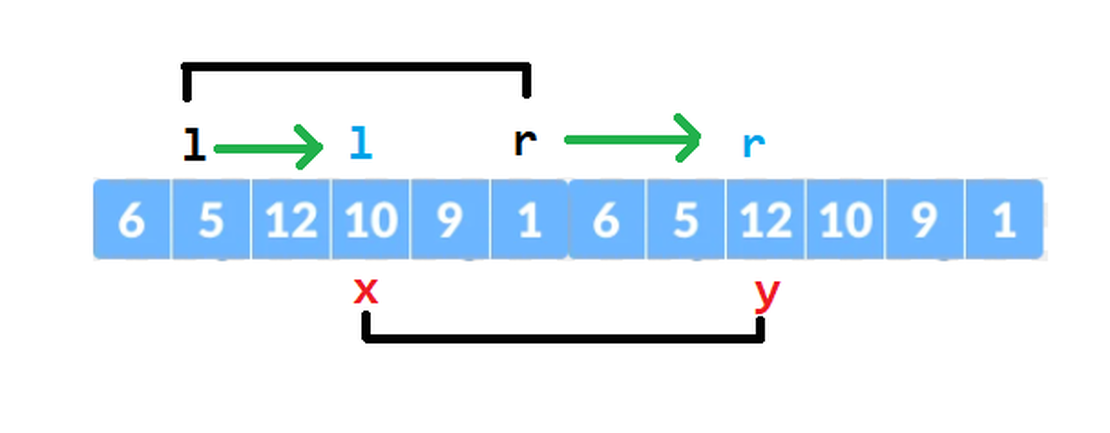
As shown below, we can exploit the overlapping region between the previous query window $[l, r]$ and the new query window $[x, y]$. We can shift our existing boundaries by moving $r \rightarrow y$ and $l \rightarrow x$, updating our unique count dynamically as the pointers slide across the array.

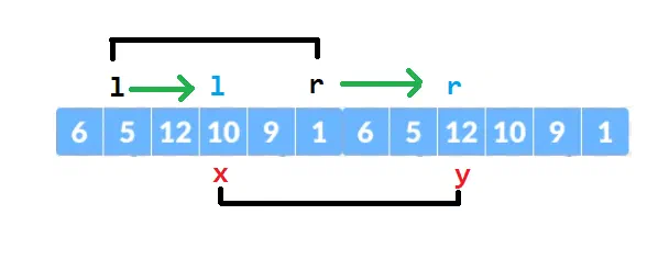
With this approach, a single query requires $| r - y | + | l - x |$ step transitions. We maintain two global pointers, $l$ and $r$, and shift them to match the new query boundaries. We use absolute differences because we don’t know where the new $x$ and $y$ sit relative to the old window-they could be completely to the left, to the right, or nested inside.

The overall runtime for this iterative shifting approach amounts to the summation of transitions: $\sum (| r_i - r_{i-1} | + | l_i - l_{i-1} |)$. $(*)$

Enter Mo’s Algorithm

Looking closely at expression $(*)$, the total number of pointer operations depends entirely on the order in which we process the queries. Since the problem only asks us to inspect the data without modifying it (read-only queries), we can process the queries offline. This means we can read all queries upfront, sort them in an optimal order, and output the answers in the original sequence.

Mo’s Algorithm introduces a specific sorting order that minimizes pointer travel distance, keeping the sum of pointer movements incredibly small.

The algorithm works as follows:

Define the block size: $BLOCK = \sqrt{N}$.
Sort the queries primarily in ascending order of the block that $l$ belongs to (i.e., l / BLOCK).
If two queries have their left endpoints in the same block, sort them in ascending order of their right endpoints ($r$).

Here is the comparator function for sorting:

bool compare(const query &A, const query &B) {
    if (A.l / BLOCK != B.l / BLOCK)
        return A.l / BLOCK < B.l / BLOCK;
    return A.r < B.r;
}

Complexity Analysis

Let’s break down how the pointers move under this sorting order:

Queries within the same Left Block:

Suppose query $i$ and query $i-1$ share the same left block (meaning $l_i / BLOCK == l_{i-1} / BLOCK$).
Since queries within the same block are sorted by $r$, the right pointer $r$ moves monotonically from left to right. Across all queries in a single block, $r$ will travel at most $N$ steps, leading to an overall complexity of $O(N)$ for that block’s right pointer.
Meanwhile, the left pointer $l$ can move back and forth, but it is confined within a single block of size $\sqrt{N}$. For each query, it moves at most $\sqrt{N}$ steps. Over $Q$ queries, this contributes $O(Q \times \sqrt{N})$ operations.
Block Complexity: $O(Q \sqrt{N} + N)$.

Transitioning between Blocks:

When the left endpoint moves to the next block, the right pointer $r$ might have to reset and move backward or forward across the array, taking up to $O(N)$ steps.
Since there are $\sqrt{N}$ blocks in total, this full reset happens at most $\sqrt{N}$ times. The total cost of these transitions for $r$ is $O(N \times \sqrt{N})$.
The left pointer $l$ simply advances into the next block, which takes $O(\sqrt{N})$ total steps across the entire execution.
Transition Complexity: $O(N \sqrt{N})$.

Combining both scenarios, the total time complexity for pointer movement is $O((N + Q) \times \sqrt{N})$. Note that the overall runtime will also scale with the time complexity of your Add and Remove helper functions (which run in $O(1)$ here).

Implementation

Below is the full C++ implementation of Mo’s Algorithm, which achieves an Accepted (AC) verdict on the classic problem DQUERY.

#include <stdio.h>
#include <algorithm>
#include <unordered_map>

using namespace std;

const int MAXN = 3e4 + 10;
const int MAXQ = 2e5 + 10;
const int BLOCK = 175; // ~sqrt(MAXN)

struct query {
    int l, r, id;
    query(int _l = 0, int _r = 0, int _id = 0):
        l(_l), r(_r), id(_id) {};
};

int n, Q;
int a[MAXN];
int res[MAXQ];
query q[MAXQ];
int answer = 0;
unordered_map<int, int> cnt;

bool compare(const query &A, const query &B) {
    if (A.l / BLOCK != B.l / BLOCK)
        return A.l / BLOCK < B.l / BLOCK;
    return A.r < B.r;
}

void Add(int pos) {
    cnt[a[pos]]++;
    if (cnt[a[pos]] == 1) answer++;
}

void Remove(int pos) {
    cnt[a[pos]]--;
    if (cnt[a[pos]] == 0) answer--;
}

void solve() {
    int curL = 1, curR = 0;
    sort(q + 1, q + 1 + Q, compare);
    for (int i = 1; i <= Q; ++i) {
        int L = q[i].l, R = q[i].r;
        while (curL < L) Remove(curL++);
        while (curL > L) Add(--curL);
        while (curR < R) Add(++curR);
        while (curR > R) Remove(curR--);
        res[q[i].id] = answer;
    }
    for (int i = 1; i <= Q; ++i) 
        printf("%d\n", res[i]);
}

void readInput() {
    scanf("%d", &n);
    for (int i = 1; i <= n; ++i)
        scanf("%d", &a[i]);
    scanf("%d", &Q);
    for (int i = 1; i <= Q; ++i) {
        scanf("%d%d", &q[i].l, &q[i].r);
        q[i].id = i;
    }
}

int main() {
    readInput();
    solve();
    return 0;
}

Pro tip: You can reuse this solve logic as a standard template for Mo’s Algorithm. For most problems, you only need to adapt the internal logic of the Add and Remove functions to fit the specific problem constraints.

Practice Problems

Ready to test your skills? Here is an excellent compilation of problems that can be solved using Mo’s Algorithm: Everything on Mo’s Algorithm

Sqrt Decomposition and Mo's Algorithm

Sqrt Decomposition

The Problem

The Core Concept

Complexity Analysis

Implementation

Mo’s Algorithm

The Problem

The Core Concept

Naive Algorithm 1

Naive Algorithm 2

Enter Mo’s Algorithm

Complexity Analysis

Implementation

Practice Problems

References

Tags:

Share: